STA 2000笔记

统计学笔记，仅作为个人学习记录，不保证正确性。

Index

• Index
• Chapter 1: Defining and Collecting Data
  • 1.1 Variables
    • 1.1.1 Measurement Scales
  • 1.2 Population and Sample
    • 1.2.1 Parameter and Statistic
    • 1.2.2 Sources of Data
    • 1.2.3 Probability Sample
• Chapter 2: Organizing and Visualizing Variables
  • 2.1 Organizing Categorical Data
  • 2.2 Organizing Numerical Data
  • 2.3 Visualizing Categorical Data
  • 2.4 Visualizing Numerical Data
    • 2.4.1 Visualing Two Numerical Variables
• Chapter 3: Numerical Descriptive Measures
  • 3.1 Measures of Central Tendency
    • 3.1.1 Mean
    • 3.1.2 Median
    • 3.1.3 Mode
  • 3.2 Measures of Variation
    • 3.2.1 Range
    • 3.2.2 Sample Variation
    • 3.2.3 Sample Standard Deviation
    • 3.2.4 Coefficient of Variation
    • 3.2.5 Z-Score
  • 3.3 Shape of a Distribution
    • 3.3.1 Skewness
    • 3.3.2 Kurtosis
  • 3.4 Quartile Measures
    • 3.4.1 Locating Quartiles
    • 3.4.2 Interquartile Range
  • 3.5 Five Number Summary
    • 3.5.1 Relationships Among the Five Number Summary and Distribution Shape
    • 3.5.2 Boxplot
  • 3.6 Numerical Descriptive Measures for Populations
    • 3.6.1 Population Mean
    • 3.6.2 Population Variance
    • 3.6.3 Population Standard Deviation
  • 3.7 Empirical Rule
  • 3.8 Chebyshev's Rule
  • 3.9 Covariance
  • 3.10 Correlation Coefficient
    • 3.10.1 Features of the Correlation Coefficient
  • 3.11 Pitfalls in Numerical Descriptive Measures
• Chapter 4: Basic Probability
  • 4.1 Events
  • 4.2 Probability
  • 4.2.1 Three Approaches to Assigning Probability
    • 4.2.2 Simple Probability
    • 4.2.3 Joint Probability
    • 4.2.4 Marginal Probability
    • 4.2.5 General Addition Rule
    • 4.2.6 Conditional Probability
    • 4.2.7 Independent Events
    • 4.2.8 Multiplication Rule
• Chapter 5: Discrete Probability Distributions
  • 5.1 Expected Value
  • 5.2 Variance and Standard Deviation
• Chapter 6: The Normal Distribution
  • 6.1 Continuous Probability Distributions
  • 6.2 Normal Distribution
    • 6.2.1 Density Function
    • 6.2.2 Standardized Normal
    • 6.2.3 Normal Probabilities
• Chapter 7: Sampling Distributions
  • 7.1 Sample Mean Sampling Distribution
    • 7.1.1 Standard Error of the Mean
    • 7.1.2 Z-Value for Sampling Distribution of Mean
    • 7.1.3 Sampling Distribution Properties
    • 7.1.4 Central Limit Theorem
  • 7.2 Population Proportions
    • 7.2.1 Sampling Distribution of the Sample Proportion
    • 7.2.2 Z-Value for Proportions
• Chapter 8: Confidence Interval Estimation
  • 8.1 Point and Interval Estimates
  • 8.2 Confidence Intervals
• Chapter 9: Fundamentals of Hypothesis Testing: One-Sample Tests
  • 9.1 The Null Hypothesis
  • 9.2 The Alternative Hypothesis
  • 9.3 The Hypothesis Testing Process
    • 9.3.1 The Test Statistic and Critical Values
    • 9.3.2 Risks in Decision Making Using Hypothesis Testing
    • 9.3.3 Level of Significance and the Rejection Region
  • 9.4 Hypothesis Tests for the Mean
    • 9.4.1 Z Test of Hypothesis for the Mean
• Chapter 10: Two-Sample Tests and One-Way ANOVA
  • 10.1 Two-Sample Tests
    • 10.1.1 Difference Between Two Means

-----

Chapter 1: Defining and Collecting Data

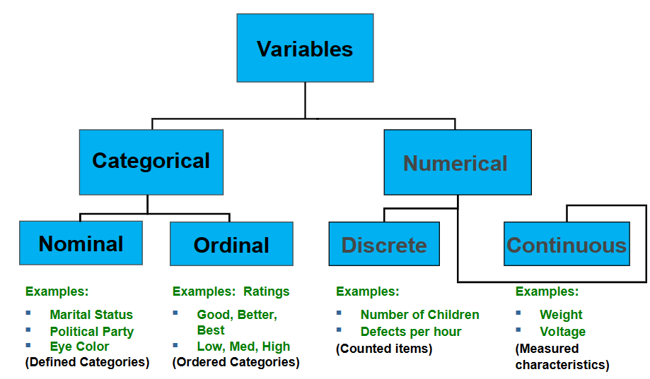
1.1 Variables

Categorical (qualitative): a variable that can be placed into a specific category, according to some characteristic or attribute.

• Nominal: no natural ordering of the categories
• Ordinal: natural ordering of the categories

Numerical (quantitative): a variable that can be measured numerically.

• Discrete: arise from a counting process
• Continuous: arise from a measuring process

1.1.1 Measurement Scales

Interval scale: an ordered scale in which the difference between measurements is a meaningful quantity but the measurements do not have a true zero point.

Ratio scale: an ordered scale in which the difference between measurements is a meaningful quantity and the measurements have a true zero point.

1.2 Population and Sample

Population: the set of all elements of interest in a particular study.

• contains all measurements of interest to the investigator

Sample: a subset of the population.

• a part of the population selected for analysis

1.2.1 Parameter and Statistic

Population parameter: a numerical measure that describes an aspect of a population.

Sample statistic: a numerical measure that describes an aspect of a sample.

1.2.2 Sources of Data

Primary sources: data that are generated by the investigator conducting the study.

• from a political survey
• collected from an experiment
• observed data

Secondary sources: data that were produced by someone other than the investigator conducting the study.

• analyzing census data
• examining data from print journals or data published on the Internet

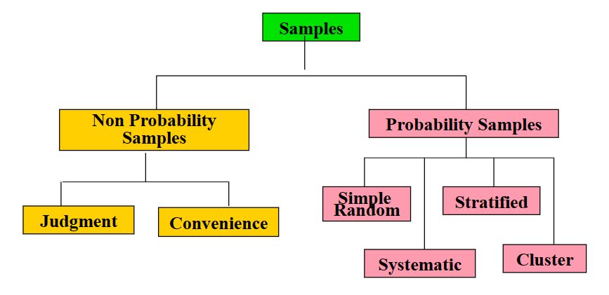
1.2.3 Probability Sample

In a probability sample, items in the sample are chosen on the basis of known probabilities.

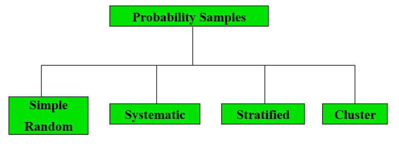
• Simple random sample: every individual or item from the frame has an equal chance of being selected
• Systematic sample: the items are selected according to a specified time or item interval in the sampling frame
  • divide frame of $N$ individuals into groups of $k$ individuals: $k=\frac{N}{n}$
• Stratified sample: divide population into two or more subgroups (strata) according to some characteristic that is important to the study
• Cluster sample: population is divided into several "clusters" or sections, then some of those clusters are randomly selected and all members of the selected clusters are used as the sample

-----

Chapter 2: Organizing and Visualizing Variables

2.1 Organizing Categorical Data

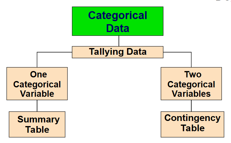
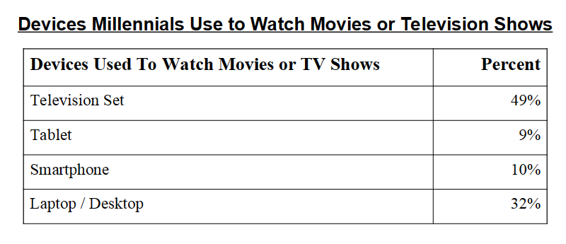
• Summary table: tallies the frequencies or percentages of items in a set of categories so that you can see differences between categories
  • 
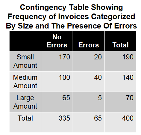
• Contingency table: a table that classifies sample observations according to two or more identifiable categories so that the relationship between the categories can be studied
  • 

2.2 Organizing Numerical Data

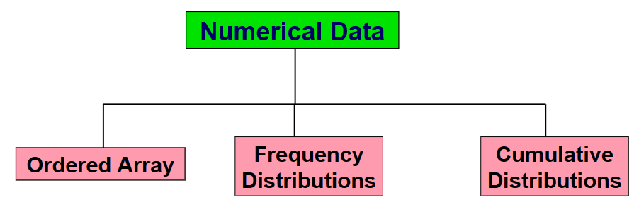
• Ordered array: a sequence of data, in rank order, from the smallest value to the largest value.
• Frequency distribution: a summary table in which the data are arranged into numerically ordered classes

2.3 Visualizing Categorical Data

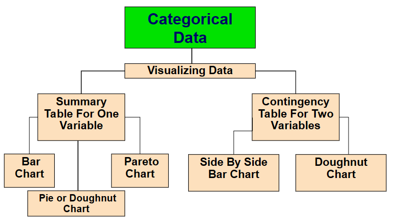
• Bar chart: visualizes a categorical variable as a series of bars
• Pie chart: a circle broken up into slices that represent categories
• Doughnut chart: the outer part of a circle broken up into pieces that represent categories
• Pareto chart: a vertical bar chart, where categories are shown in descending order of frequency
• Side by side bar chart: a bar chart that compares two or more categories
• Doughnut chart (contingency): a doughnut chart that compares two or more categories

2.4 Visualizing Numerical Data

• Stem-and-leaf display: a simple way to see how the data are distributed and where concentrations of data exist
• Histogram: a vertical bar chart of the data in a frequency distribution
• Percentage polygon: formed by having the midpoint of each class represent the data in that class and then connecting the sequence Of midpoints at their respective class percentages

2.4.1 Visualing Two Numerical Variables

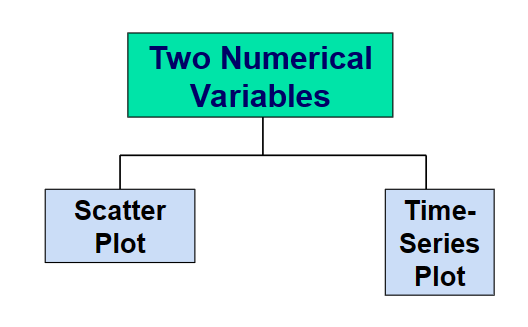
• Scatter plot: used for numerical data consisting of paired observations taken from two numerical variables
• Time series plot: used to study patterns in the values of a numeric variable over time

-----

Chapter 3: Numerical Descriptive Measures

Central tendency: the extent or inclination to which the values of a numerical variable group or cluster around a typical or central value.

3.1 Measures of Central Tendency

Measure of central tendency: a single value that attempts to describe a set of data by identifying the central position within that set of data.

3.1.1 Mean

$$\bar{X} = \frac{\sum_{i=1}^{n} X_i}{n} = \frac{X_1 + X_2 + \cdots + X_n}{n}$$

• $\bar{X}$ -> sample mean; pronounced "X-bar"
• $n$ -> sample size
• $X_i$ -> the $i$th value in the sample
• $X_n$ -> the observed values

3.1.2 Median

1. Sample size is odd:

$$\text{Median} = \frac{x+1}{2}^{th} \text{position}$$

2. Sample size is even:

$$\text{Median} = \frac{n}{2}^{th} \text{and} \frac{n}{2} + 1^{th} \text{positions}$$

3.1.3 Mode

Mode: the value that occurs most frequently in a data set.

3.2 Measures of Variation

Measure of variation: gives information on the spread or variability or dispersion of the data values.

3.2.1 Range

$$\text{Range} = \text{Maximum} - \text{Minimum}$$

3.2.2 Sample Variation

Sample variance: average of squared deviations of values from the mean.

$$S^2 = \frac{\sum_{i=1}^{n} (X_i - \bar{X})^2}{n-1}$$

• $\bar{x}$ -> arithmetic mean
• $n$ -> sample size
• $X_i$ -> the $i$th value in the sample

3.2.3 Sample Standard Deviation

$$S = \sqrt{\frac{\sum_{i=1}^{n} (X_i - \bar{X})^2}{n-1}}$$

3.2.4 Coefficient of Variation

$$CV = \frac{S}{\bar{X}} \times 100\%$$

3.2.5 Z-Score

Z-Score: the number of standard deviations that a given value $X$ is above or below the mean.

• a data value is considered an extreme outlier if its Z-Score is less than -3 or greater than +3

$$Z = \frac{X - \bar{X}}{S}$$

3.3 Shape of a Distribution

3.3.1 Skewness

Skewness: a measure of the degree of asymmetry of a distribution.

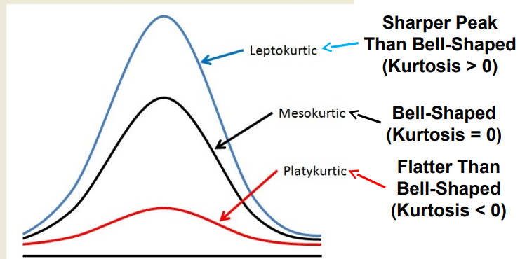
3.3.2 Kurtosis

Kurtosis: a measure of the degree of peakedness of a distribution.

3.4 Quartile Measures

Quartile: a value that divides a data set into four groups containing (as far as possible) an equal number of observations.

• $Q_1$ -> first quartile
• $Q_2$ -> second quartile; the median
• $Q_3$ -> third quartile

3.4.1 Locating Quartiles

1. $Q_1 = \frac{n+1}{4}$ ranked value
2. $Q_2 = \frac{n+1}{2}$ ranked value
3. $Q_3 = \frac{3(n+1)}{4}$ ranked value

• $n$ -> the number of observed values

3.4.2 Interquartile Range

Interquartile range: the difference between the third and first quartiles.

$$IQR = Q_3 - Q_1$$

3.5 Five Number Summary

Five number summary: the five numbers that help describe the center, spread and shape of data.

• $\text{minimum}$
• $Q_1$
• $Q_2$ / Median
• $Q_3$
• $\text{maximum}$

3.5.1 Relationships Among the Five Number Summary and Distribution Shape

Left-Skewed	Symmetric	Right-Skewed
$Median - \text{minimum} > \text{maximum} - Median$	$Median - \text{minimum} \approx \text{maximum} - Median$	$Median - \text{minimum} < \text{maximum} - Median$
$Q_1 - \text{minimum} > \text{maximum} - Q_3$	$Q_1 - \text{minimum} \approx \text{maximum} - Q_3$	$Q_1 - \text{minimum} < \text{maximum} - Q_3$
$Median - Q_1 > Q_2 - Median$	$Median - Q_1 \approx Q_2 - Median$	$Median - Q_1 \approx Q_2 - Median$

3.5.2 Boxplot

Boxplot: a graphical display of the five number summary.

3.6 Numerical Descriptive Measures for Populations

3.6.1 Population Mean

$$\mu = \frac{\sum_{i=1}^{N} X_i}{N}$$

• $\mu$ -> population mean
• $N$ -> population size
• $X_i$ -> the $i$th value in the population

3.6.2 Population Variance

$$\sigma^2 = \frac{\sum_{i=1}^{N} (X_i - \mu)^2}{N}$$

3.6.3 Population Standard Deviation

$$\sigma = \sqrt{\frac{\sum_{i=1}^{N} (X_i - \mu)^2}{N}}$$

3.7 Empirical Rule

Empirical rule: approximates the variation of data in a symmetric mound-shaped distribution.

• 68% of the data values lie within one standard deviation of the mean
• 95% of the data values lie within two standard deviations of the mean
• 99.7% of the data values lie within three standard deviations of the mean

3.8 Chebyshev's Rule

Chebyshev's rule: applies to any data set, regardless of the shape of the distribution.

• at least $1-\frac{1}{k^2}$ of the data values lie within $k$ standard deviations of the mean, where $k$ is any value greater than 1

3.9 Covariance

Covariance: a measure of the linear association between two variables.

$$Cov(X,Y) = \frac{\sum_{i=1}^{n} (X_i - \bar{X})(Y_i - \bar{Y})}{n-1}$$

• $Cov(X,Y) > 0$ -> positive covariance; as $X$ increases, $Y$ increases
• $Cov(X,Y) < 0$ -> negative covariance; as $X$ increases, $Y$ decreases
• $Cov(X,Y) = 0$ -> no linear relationship between $X$ and $Y$

3.10 Correlation Coefficient

Correlation coefficient: a measure of the linear association between two variables.

$$r = \frac{Cov(X,Y)}{S_X S_Y}$$

• $Cov(X,Y) = \frac{\sum_{i=1}^{n} (X_i - \bar{X})(Y_i - \bar{Y})}{n-1}$
• $S_X = \sqrt{\frac{\sum_{i=1}^{n} (X_i - \bar{X})^2}{n-1}}$
• $S_Y = \sqrt{\frac{\sum_{i=1}^{n} (Y_i - \bar{Y})^2}{n-1}}$

3.10.1 Features of the Correlation Coefficient

The population coefficient of correlation, $\rho$, is a measure of the linear association between two variables.

The sample coefficient of correlation, $r$, is a measure of the linear association between two variables.

3.11 Pitfalls in Numerical Descriptive Measures

• Data analysis is objective
• Data interpretation is subjective

-----

Chapter 4: Basic Probability

Sample space: the set of all possible outcomes of an experiment.

4.1 Events

Simple event: an event described by a single characteristic or an event that is a set of outcomes of an experiment.

Joint event: an event described by two or more characteristics.

Complement of an event A:

• all events that are not part of event A

4.2 Probability

Probability: the numerical value representing the chance, likelihood, or possibility that a certain event will occur.

• always between 0 and 1

Impossible event: an event that has no chance of occurring.

Certain event: an event that is sure to occur.

Mutually exclusive events: events that cannot occur at the same time.

Collectively exhaustive events: the set of events that covers the entire sample space.

• one of the events must occur

4.2.1 Three Approaches to Assigning Probability

A priori probability: a probability assignment based upon prior knowledge of the process involved.

• $P(A) = \frac{\text{number of outcomes in A}}{\text{total number of outcomes}}$
• Example: randomly selecting a day from the year 2019. What is the probability that the day is in January?
  • $P(\text{January}) = \frac{31}{365}$

Empirical probability: a probability assignment based upon observations obtained from probability experiments.

• $P(A) = \frac{\text{number of times A occurs}}{\text{number of times the experiment is repeated}}$
• Example: $P(\text{male taking stats}) = \frac{\text{number of males taking stats}}{\text{total number of people}}$

Subjective probability: a probability assignment based upon judgment.

• $P(A) = \frac{\text{degree of belief that A will occur}}{\text{degree of belief that A will occur} + \text{degree of belief that A will not occur}}$
• differs from person to person

4.2.2 Simple Probability

Simple probability: the probability of a single event occurring.

$$P(A) = \frac{\text{number of outcomes satisfying A}}{\text{total number of outcomes}}$$

4.2.3 Joint Probability

Joint probability: the probability of two or more events occurring simultaneously.

$$P(A \cap B) = \frac{\text{number of outcomes satisfying A and B}}{\text{total number of outcomes}}$$

4.2.4 Marginal Probability

Marginal probability: the probability of a single event occurring without regard to any other event.

$$P(A) = \frac{\text{number of outcomes satisfying A}}{\text{total number of outcomes}} = P(A \cap B) + P(A \cap B^c)$$

	$B$	$B^c$	Total
$A$	$P(A \cap B)$	$P(A \cap B^c)$	$P(A)$
$A^c$	$P(A^c \cap B)$	$P(A^c \cap B^c)$	$P(A^c)$
Total	$P(B)$	$P(B^c)$	1

• $P(A \cap B)$ and $P(A \cap B^c)$ are joint probabilities
• $P(A^c)$ and $P(B^c)$ are marginal probabilities

4.2.5 General Addition Rule

General addition rule: the probability of the union of two events is the sum of the probabilities of the two events minus the probability of their intersection.

$$P(A \cup B) = P(A) + P(B) - P(A \cap B)$$

If $A$ and $B$ are mutually exclusive, then $P(A \cap B) = 0$. Therefore, the general addition rule becomes:

$$P(A \cup B) = P(A) + P(B)$$

4.2.6 Conditional Probability

Conditional probability: the probability of an event occurring given that another event has already occurred.

1. The condition probability of $A$ given that $B$ has occured:

$$P(A|B) = \frac{P(A \cap B)}{P(B)}$$

2. The condition probability of $B$ given that $A$ has occured:

$$P(B|A) = \frac{P(A \cap B)}{P(A)}$$

• where $P(A \cap B)$ is the joint probability of $A$ and $B$
  • $P(A)$ -> marginal probability of $A$
  • $P(B)$ -> marginal probability of $B$

4.2.7 Independent Events

Independent events: two events are independent if the occurrence of one event does not affect the probability of the occurrence of the other event.

$$P(A|B) = P(A) \space \text{;} \space P(B|A) = P(B)$$

• events $A$ and $B$ are independent when the probability of one event is not affects by the fact that the other event has occurred

4.2.8 Multiplication Rule

Multiplication rule: the probability of the intersection of two events is the product of the probability of the first event and the conditional probability of the second event given that the first event has occurred.

$$P(A \cap B) = P(A) \times P(B|A)$$

$$P(A|B) = \frac{P(A \cap B)}{P(B)} = \frac{P(A) \times P(B|A)}{P(B)}$$

If $A$ and $B$ are independent, then $P(B|A) = P(B)$, and the multiplication rule becomes:

$$P(A \cap B) = P(A) \times P(B)$$

-----

Chapter 5: Discrete Probability Distributions

Probability distribution: a listing of all the outcomes of an experiment and the probability associated with each outcome.

5.1 Expected Value

Expected value: the mean of a probability distribution -> $\mu$.

$$\mu = \sum_{i=1}^{n} x_i P(x_i)$$

• $x_i$ -> the $i$th value in the probability distribution
• $P(x_i)$ -> the probability associated with the $i$th value in the probability distribution
• $n$ -> the number of values in the probability distribution
• $\mu$ -> the expected value

5.2 Variance and Standard Deviation

Variance: the average of the squared deviations of the possible values from the expected value.

$$\sigma^2 = \sum_{i=1}^{n} (x_i - \mu)^2 P(x_i)$$

• $x_i$ -> the $i$th value in the probability distribution
• $P(x_i)$ -> the probability associated with the $i$th value in the probability distribution
• $n$ -> the number of values in the probability distribution

Standard deviation: the square root of the variance.

-----

Chapter 6: The Normal Distribution

6.1 Continuous Probability Distributions

Continuous variable: a variable that can assume any value on a continuum (can assume an uncountable number of values)

For example, the thickness of an item, the time required to complete a task.

6.2 Normal Distribution

Normal Distribution:

• bell shaped
• symmetrical
• mean, median and mode are equal

The location is determined by the mean, $\mu$, and the spread is determined by the standard deviation, $\sigma$.

The random variable has an infinite theoretical range: $(-\infty, \infty)$.

6.2.1 Density Function

Probability density function: a function whose integral is calculated to find probabilities associated with a continuous random variable.

$$f(x) = \frac{1}{\sigma \sqrt{2\pi}} e^{-\frac{1}{2}(\frac{x-\mu}{\sigma})^2}$$

• $e$ -> the mathematical constant approximately equal to 2.71828
• $\pi$ -> the mathematical constant approximately equal to 3.14159
• $\mu$ -> the mean of the distribution
• $\sigma$ -> the standard deviation of the distribution
• $x$ -> the value of the continuous variable

6.2.2 Standardized Normal

Standardized normal distribution: a normal distribution with a mean of 0 and a standard deviation of 1.

$$z = \frac{x-\mu}{\sigma}$$

Its density function is:

$$f(z) = \frac{1}{\sqrt{2\pi}} e^{-\frac{1}{2}z^2}$$

• $e$ -> the mathematical constant approximately equal to 2.71828
• $\pi$ -> the mathematical constant approximately equal to 3.14159
• $z$ -> the standardized value of the continuous variable

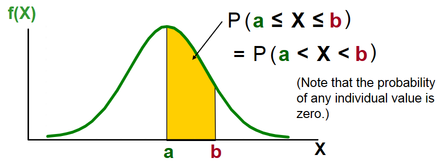
6.2.3 Normal Probabilities

Probability is measured by the area under the curve.

Uniform Distribution: a continuous probability distribution in which the probability of observing a value x in any interval of equal length is the same for each interval of the same length. Also known as rectangular distribution.

Exponential Distribution: a continuous probability distribution that is used to describe the time between events that occur at a constant average rate and are independent of each other. The exponential distribution is skewed to the right.

-----

Chapter 7: Sampling Distributions

Sampling distribution: a distribution of all of the possible values of a sample statistic for a given sample size selected from a population.

$$\bar{X} = \frac{\sum_{i=1}^{n} X_i}{n}$$

Assume there is a population:

• population size $N=4$
• variable of interest is, $X$, age of individuals
• values of $X$: $18, 20, 22, 24$ (years)

$$\mu = \frac{18+20+22+24}{4} = 21$$

$$\sigma = \sqrt{\frac{\sum^n_{i=1}(X_i-\mu)^2}{N}} = 2.236$$

7.1 Sample Mean Sampling Distribution

7.1.1 Standard Error of the Mean

Standard error of the mean: the standard deviation of the sampling distribution of the sample mean.

$$\sigma_{\bar{X}} = \frac{\sigma}{\sqrt{n}}$$

7.1.2 Z-Value for Sampling Distribution of Mean

$$Z = \frac{\bar{X}-\mu}{\sigma_{\bar{X}}} = \frac{\bar{X}-\mu}{\frac{\sigma}{\sqrt{n}}}$$

• $\bar{X}$ -> sample mean
• $\mu$ -> population mean
• $\sigma_{\bar{X}}$ -> standard error of the mean

7.1.3 Sampling Distribution Properties

• The mean of the sampling distribution of the sample mean is equal to the mean of the population
• As $n$ increases, the standard error of the mean ($\sigma_{\bar{X}}$) decreases

$$\mu_{\bar{X}} = \mu$$

7.1.4 Central Limit Theorem

Central limit theorem: the sampling distribution of the sample mean is approximately normal for a sufficiently large sample size.

• as the sample size gets large enough, the sampling distribution of the sample mean becomes almost normal regardless of shape of population

Central limit theorem is used when the population is not normal.

How large is large enough?

• for most distributions, $n \gt 30$ is sufficient
• for fairly symmetric distributions, $n \gt 15$ is sufficient
• for a normal population distribution, the sampling distribution of the sample mean is always normally distributed

7.2 Population Proportions

$\pi$: the proportion of the population having some characteristic.

Sample proportion ($p$): provides an estimate of $\pi$:

$$p = \frac{\text{number of items in the population having the characteristic}}{\text{total number of items in the population}}$$

• $0 \leq p \leq 1$
• $p$ is approximately distributed as a normal distribution when $n$ is large

7.2.1 Sampling Distribution of the Sample Proportion

$$\sigma_p = \sqrt{\frac{\pi(1-\pi)}{n}}$$

• $\pi$ -> population proportion
• $n$ -> sample size
• $\sigma_p$ -> standard error of the sample proportion
• $p$ -> sample proportion

7.2.2 Z-Value for Proportions

$$Z = \frac{p-\pi}{\sigma_p} = \frac{p-\pi}{\sqrt{\frac{\pi(1-\pi)}{n}}}$$

-----

Chapter 8: Confidence Interval Estimation

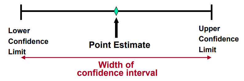
8.1 Point and Interval Estimates

Point estimate: a single number.

Confidence interval: a set of two plausible values at a specified confidence level that contains true parameter.

8.2 Confidence Intervals

Interval estimate: provides more information about a population characteristic than does a point estimate -> confidence intervals.

-----

Chapter 9: Fundamentals of Hypothesis Testing: One-Sample Tests

Hypothesis: a claim or assertion about a population parameter.

Example:
The mean diameter of a manufactured bolt is $30$mm -> $H_0:\mu=30$

9.1 The Null Hypothesis

• begin with the assumption that the null hypothesis is true
• similar to the notion of innocent until proven guilty
• represents the current belief in a situation
• always contains $=$, or $\leq$, or $\geq$ sign
• may or may not be rejected

9.2 The Alternative Hypothesis

• is the opposite of the null hypothesis
• the mean diameter of a manufactured bolt is not equal to $30$mm
• challenges the status quo
• never contains the $=$, or $\leq$, or $\geq$ sign
• may or may not be proven
• is generally the hypothesis that the researcher is trying to prove

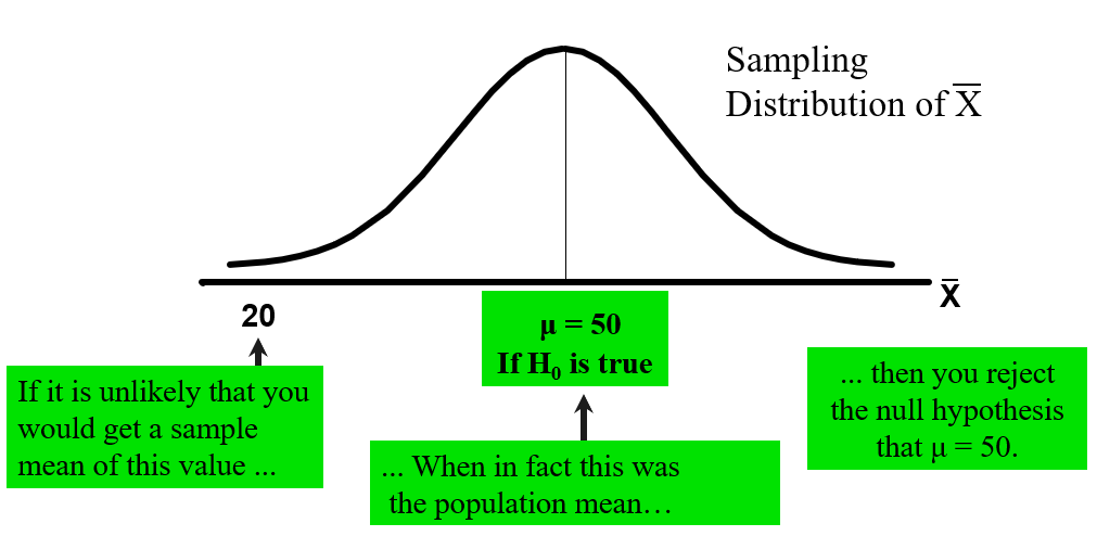
9.3 The Hypothesis Testing Process

The population mean age is $50$.

• $H_0: \mu = 50$
• $H_1: \mu \neq 50$

Suppose the sample mean age was $\bar{X} = 20$.
This is lower than the claimed mean population age of $50$.

If the null hypothesis were true, the probability of getting such a different sample mean would be very small, so you reject the null hypothesis.

In other words, getting a sample mean of $20$ is so unlikely if the population mean was $50$, you conclude that the population mean must not be $50$.

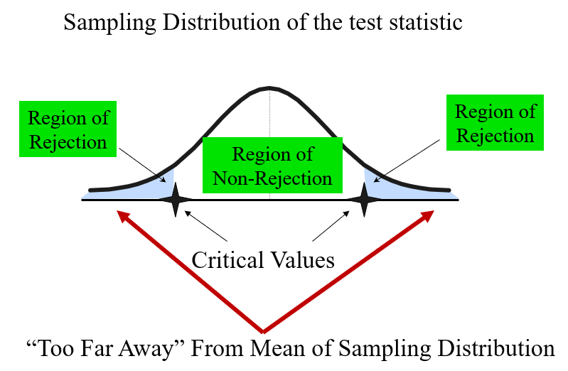
9.3.1 The Test Statistic and Critical Values

If the sample mean is close to the stated population mean, the null hypothesis is not rejected.

If the sample mean is far from the stated population mean, the null hypothesis is rejected.

How far is "far enough" to reject $H_0$?

The critical value of a test statistic creates a "line in the sand" for decision making -- it answers the question of how far is far enough.

9.3.2 Risks in Decision Making Using Hypothesis Testing

• Type I error: rejecting the null hypothesis when it is true
  • a "false alarm"
  • the probability of a Type I Error is $\alpha$
    • called level of significance of the test
    • set by researcher in advance
• Type II error: failing to reject the null hypothesis when it is false
  • a "missed opportunity"
  • the probability of a Type II Error is $\beta$

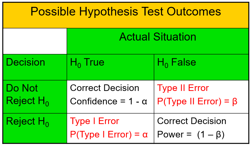
• the confidence coefficient is $(1-\alpha)$: the probability of not rejecting $H_0$ when it is true
• the confidence level of a hypothesis test is $(1-\alpha)\times 100 \%$
• the power of a statistical test $(1-\beta)$ is the probability of rejecting $H_0$ when it is false

Type I and Type II errors cannot happen at the same time.

• A Type I error can only occur if $H_0$ is true
• A Type II error can only occur if $H_0$ is false

Factors affecting Type II Error:
All else equal ...

• $\beta \uparrow$ when the difference between hypothesized parameter and its true value $\downarrow$
• $\beta \uparrow$ when $\alpha \downarrow$
• $\beta \uparrow$ when $\sigma \uparrow$
• $\beta \uparrow$ when $n \downarrow$

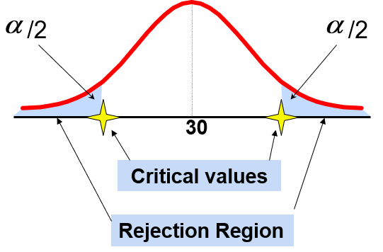
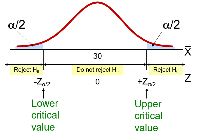
9.3.3 Level of Significance and the Rejection Region

$H_0: \mu = 30$
$H_1: \mu \neq 30$
Level of significance = $\alpha$

This is a two-tail test because there is a rejection region in both tails.

9.4 Hypothesis Tests for the Mean

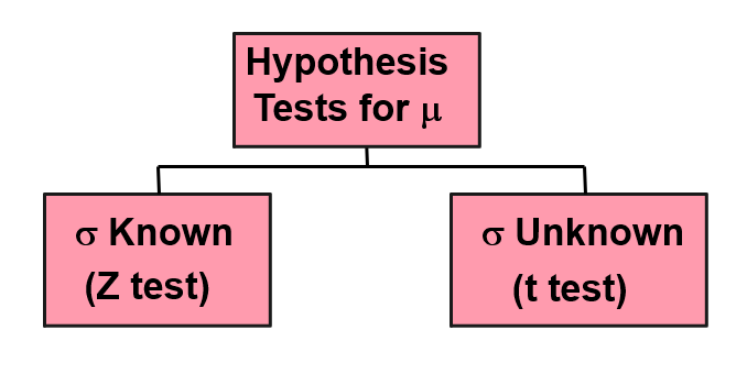
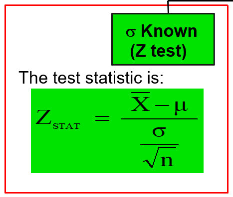
9.4.1 Z Test of Hypothesis for the Mean

Convert sample statistic ($\bar{X}$) to a $Z_{\text{STAT}}$ test statistic.

For a two-tail test for the mean, $\sigma$ known:

• determine the critical $Z$ values for a specified level of significance $\alpha$ from a table or by using computer software
  Decision rule: if the test statistic falls in the rejection region, reject $H_0$ otherwise do not reject $H_0$

-----

Chapter 10: Two-Sample Tests and One-Way ANOVA

10.1 Two-Sample Tests

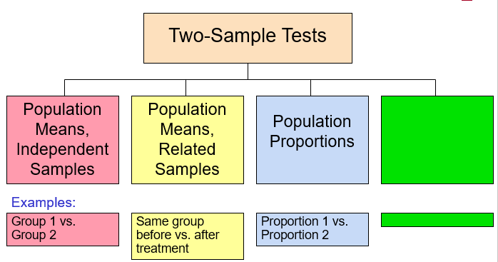
10.1.1 Difference Between Two Means

To test hypothesis or form a confidence interval for the difference between two population means, $\mu_1 - \mu_2$.

The point estimate for the difference is:
$\bar{X}_1 - \bar{X}_2$